Bipedal Walking Using RL: Deep Dive with Code
Introduction
Humanoids are the ultimate physical embodiment of AI, and represent an important playground to test the limitations of current learning algorithms as well as a critical benchmark to reference with the most general purpose cognitive embodiment we know of: humans.
One of the biggest challenges of bringing humanoid robots into the physical world, is building human level bipedal controllers that can generalize to random environments like hills/snow/stairs, master multi-skill policies like walking/running/jogging, robust to failures, and being energy efficient to perform long horizon tasks.
In this blog, we will go over the biomechanics of walking, limitations of classical control theory like Model Predictive Controllers, how reinforcement learning fixes this and how we apply our techniques to train a UniTree G1 bipedal robot in Isaac Gym with sim2sim evaluation in Mujoco.
Biomechanics of Walking
If you’ve ever taken a mechanical vibration course, you’d know that a lot of complex dynamic systems can be simplified and modeled with elastic springs.
In its simplest form, we can think of humanoid walking as balancing an inverted pendulum with springs that store/output energy by alternating kinetic/potential energy (in a friction free world this is known as passive dynamics).
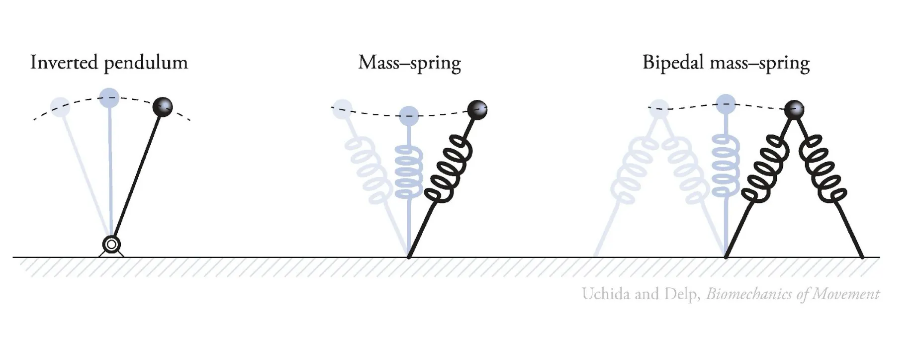
However, in reality using such simple dynamic models for control will fail immediately when deployed into the physical world. The reality is, we have not accounted for non-linear friction, randomized terrains, ability to withstand perturbations, and so on.
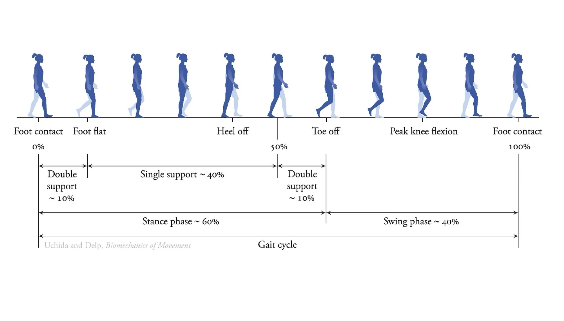
The following is a detailed figure of a typical human walking gait cycle to visualize intuitively the kind of problem we’re solving1:
We can go one step further from the simplified inverted pendulum model and actually model each leg with six degrees of freedom (DoF)2, which is the model estimates used by many humanoid robot companies:
- Hip: yaw + roll + pitch = 3 DoF
- Knee: pitch = 1 DoF
- Ankle: pitch + roll = 2 DoF
In fact, we’re able to actually derive the dynamic equations of bipedal robots using these estimates with Lagrangian dynamics, and use the well understood Model-Predictive Control (MPC) toolbox to control our bipedal locomotion3.
Dynamics of how the leg moves and should move is relatively a solved problem, humanoid and legged robotic companies have pretty much solved the teleoperation problem of robots. However, when it comes to deploy these robots into the real world: how the robot should sequence its legs, how long/strong should it swing its leg, this is a very high dimensional space and its really hard to come up with a good solutions using classical control.
Limitations of Classical Controllers
As it turns out – non-linear models take a lot of time to solve, our system is under-actuated, the models are very simplified and don’t capture the full possible legged dynamics, and finally it is extremely hard to figure out the optimal hyper-parameters that could perform well in a generalized form in the complex real world.
Moreover, building a general purpose bipedal controller requires solving for multi-objective control optimizations, we need to simultaneously solve for stability, energy efficiency, speed, and natural gaits.
Which makes this problem suitable to solve using reinforcement learning!
Reinforcement Learning for Locomotion
At the heart of training with RL is data. It’s all about generating data to show how the robot can interact with the environment i.e. world model, and then using that data to train an agent. In RL, our model is an agent and it learns through its experiences.
RL works best when we are able to make real world distribution become part of the training data distribution. I really like this analogy4 made by Jim Fan from Nvidia during his recent talk at Sequoia Capital: “simulation principle is mapping from 1,000,000 to 1,000,001st” meaning the real world should look very similar to what we have in our training set.
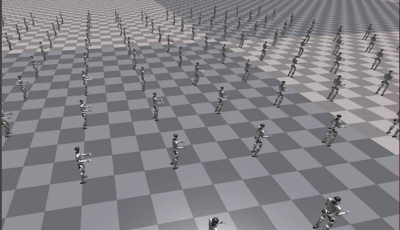
Therefore, the best control policies are those that can massively benefit from training in parallel environments and leverage GPUs; and design rewards that benefit from parallelization.
Moreover, given the nature of humanoid companies where they have large fleets of robots, it’s essential to train a control policy that can account for all the physical variances between robots and deployed from one-to-all in one shot. Which is why parallelization can learn this effectively because we can randomize each scene with different physical parameters and learn a generalized policy from all experiences.
RL Formulation for Bipedal Walking
To formalize how RL is applied to bipedal walking, we can break it down into 4 key components that are part of any RL problem:
- State Space:
- joint positions and velocities
- body orientation (roll, pitch, yaw)
- center of mass position and velocity
- contact sensors (binary signals indicating foot contact)
- command signals (desired velocity, direction)
- Action Space:
- commanded joint positions/torques for each actuator
- Reward Function:
- accounts for things like energy efficiency, speed, failure recovery, etc.
- Policy Network Architecture:
- observation encoder (fully connected layers)
- memory component (GRU/LSTM) to handle temporal dependencies
- actor network (outputs actions)
- critic network (estimates value function)
PPO for Bipedal Walking
Proximal Policy Optimization (PPO) has become the go-to algorithm for training legged robots for several reasons:
- Sample Efficiency: compared to other policy gradient methods, PPO makes better use of collected experience through multiple update epochs
- Stability: the clipped objective function prevents destructively large policy updates
- Parallelization: PPO can efficiently utilize thousands of parallel environments to collect diverse experiences
- Simple Implementation: compared to more complex algorithms like SAC or TD3, PPO has fewer hyperparameters and is more forgiving
A simplified PPO training loop for bipedal walking looks something like like:
for iteration in range(num_iterations):
    # Collect experience using current policy
    trajectories = collect_trajectories(policy, environments)

    # Compute advantages and returns
    advantages = compute_gae(trajectories, value_function)

    # Update policy using PPO objective
    for epoch in range(num_epochs):
        for mini_batch in mini_batches(trajectories):
            update_policy(mini_batch, advantages)
            update_value_function(mini_batch)

    # Adjust environment difficulty i.e. curriculum
    if mean_reward > threshold:
        increase_difficulty(environments)
Something I’ve noticed while reading lots of papers training legged robots is that the RL algorithm doesn’t change that much nor does it make significant improvements per se, as much as spending time on the training setup in simulation. This observation has also been replicated with recent advancements applying RL to LLMs, where the RL algorithms are still the same but priors and reasoning have significantly improved5.
Observation and Action Processing
A critical aspect often overlooked in RL for locomotion is proper observation and action processing:
- Observation Normalization: standardizing observations (zero mean, unit variance) across different dimensions helps stabilize training. This is especially important for bipedal robots where sensor values have different scales (angles vs. velocities).
- Action Clipping and Scaling: actions need proper scaling to match the robot’s physical limitations:
def process_actions(raw_actions): # Scale from [-1,1] to actual joint limits scaled_actions = raw_actions * action_scale # Add safety clipping clipped_actions = np.clip(scaled_actions, joint_min_limits, joint_max_limits) return clipped_actions - Phase-Based Control: many successful implementations use phase variables (cyclical values indicating where in the gait cycle the robot is) to help the policy learn periodic behaviours.
If you’re ever feel like doing everything right yet not seeing your robot learn properly, make sure that you got your observations and action processing properly! Ideally, I’ve found it best to get this done at the early stages of training by taking an overfit than regularize approach in order to trust your entire training infrastructure.
Rewards for Walking
One of the most intuitive ways I found to think about crafting rewards for robot locomotion is to think of it as generating supervised learning data where we engineer the labeled data through our rewards, simulation setup, etc. This means that more effort spent on crafting a general reward function means high quality data.
Some important rewards to include as part of your overall reward function to optimize for during training are:
- not falling
- walking at certain periodicity
- symmetry
- smoothness
- adhering to commands
- energy efficiency
- etc
Designing reward functions is a topic that deserves its own blog! For the purposes of this blog, checkout the experiments section of this blog and code to see how we’ve constructed a simple reward function for walking.
Performance Metrics
Although this is not an exhaustive list, these are some high level metrics to look out for when training bipedal robots6:
- forward velocity
- energy per meter
- time to fall
- success on push-recovery perturbations tests
- etc.
While training walking policies, you’d typically look at other metrics like average length per episode, reward direction (is it increasing overall), etc.
Symmetry Exploitation
Bipedal robots have an inherent symmetry that can be exploited:
- Mirrored Experiences: converting experiences from left to right and vice versa can effectively double our training data
- Symmetric Policy Architecture: using network architectures that enforce symmetric responses for symmetric situations
- Reward Symmetry: ensuring the reward function doesn’t favour one leg over the other
Exploration Strategies
For bipedal locomotion, engineering exploration is crucial:
- Action Noise Decay: starting with high exploration noise and gradually decreasing it allows the policy to first explore the action space broadly, then refine its own movements
- Reference Motion Bias: initializing exploration around motion primitives from mocap data or simple controllers can accelerate learning
- Curriculum-Based Exploration: adapting the noise level based on the environment difficulty helps maintain an appropriate exploration level throughout training
Challenges of Reinforcement Learning
While RL offers an immense leverage to build human level bipedal locomotion controllers, there are still critical challenges in order to build general purpose models. Some of them include:
- Reward Design: design rewards by hand to solve for the multi-objectives required
- Multi-Policies: how to have a walk, run, jog, and so on with one unified controller
- Encoding Human Style and motion into walking
- Generalization to challenging terrains (snow, ice, steep hills, etc)
Also, it’s hard to trust RL training results immediately and assume that certain methods don’t work. Because not scaling environment parallelization means less exploration, getting curriculum learning wrong means the robot might have to master complex tasks before learning the basics, and so forth.
Experiments
In my experiments, I was training on my 4GB NVIDIA GTX 1650 GPU, which is much smaller compared to what most research projects use or even training infrastructure of robotics companies.
Even with limited hardware, results can sufficiently improve by adjusting parameters and managing exploration vs. exploitation carefully.
After doing hundreds of training runs with RL for different types of legged robots like Spot, Cassie, and UniTree’s I’ve found that the best way to build a production grade RL controller for bipedal robots should look something like this:
- Simulation Maxing: I’ve found that, for the time being, training in Isaac Lab to be the most effective to build real world controllers. You can parallelize training runs massively = exploration, leverage GPUs for compression 10,000 humans hours into 2hrs simulations, ramp up iterations = exploitation, and use many existing projects as references to apply domain randomizations
- Sim2Sim Evals: have a coding infrastructure that makes it super easy to go from training in Isaac Gym to testing in Mujoco (or any other sophisticated physics engine) is critical to build at the beginning. Moreover, building some kinds of benchmarks that test these policies in different terrains before they’re deployed into physical world
- Sim2Real: although I didn’t experiment much with this in these experiments, I’ve worked on this problem more during my time at Inria as well as my first time job. I think early on, even though teleoperation isn’t the end goal being confident that your robots can track motions accurately and receive the right signals and perform what they’re told is very important too. this will help you make sure you’ve tuned/modeled your actuators properly. if you want to learn more about sim2real, read here
Training Runs
All of the training runs I did was using PPO as the RL algorithm.
1) Initial Test Run
python legged_gym/scripts/train.py --task=g1 --experiment_name=g1_test --num_envs=128 --max_iterations=100 --seed=42
- Parameters: 128 parallel environments, 100 iterations
- Results:
- mean reward: 0.02
- mean episode length: 32.32 steps
- training time: ~10 minutes
- robot behaviour: robots could barely stand before falling over
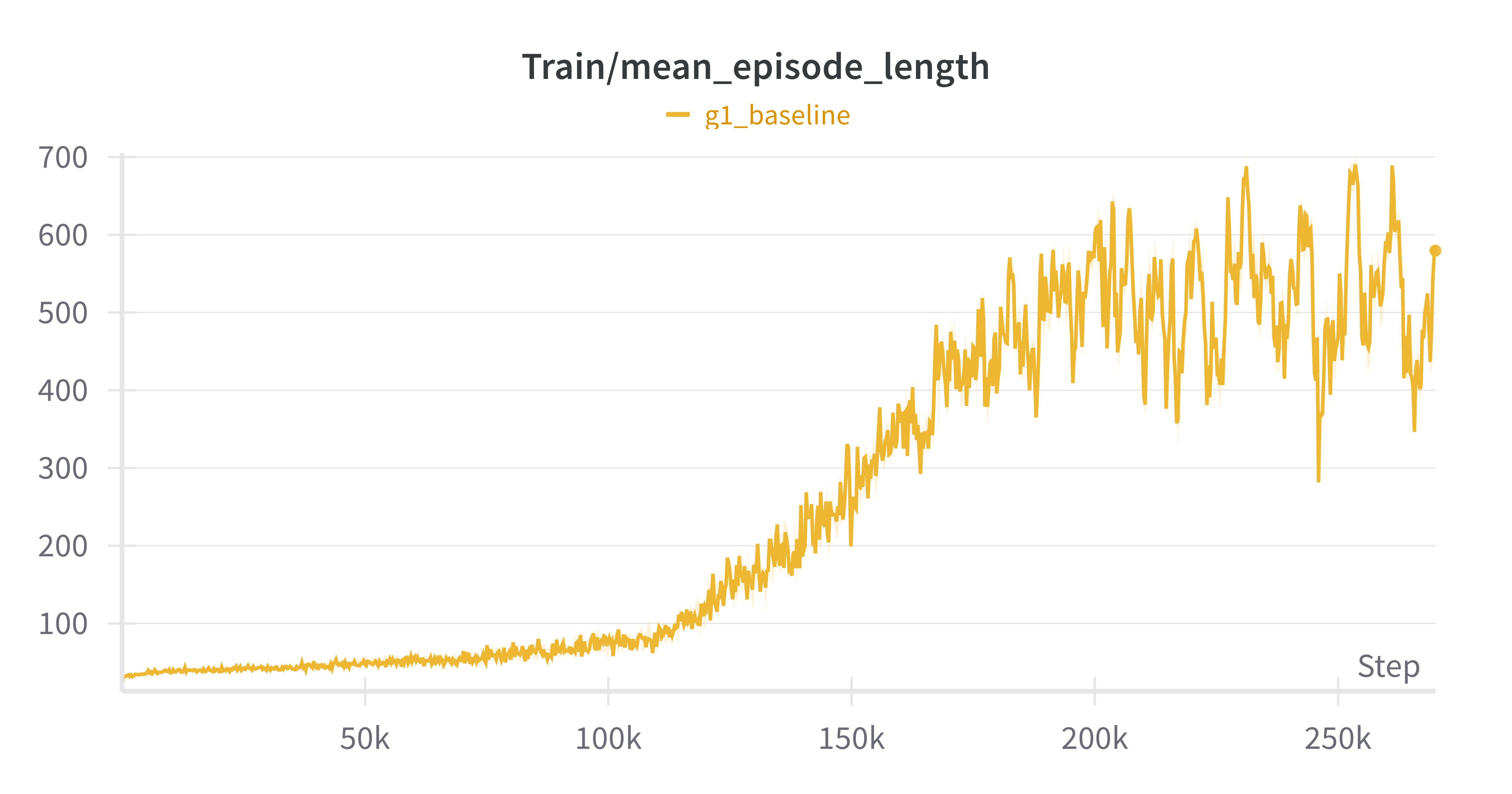
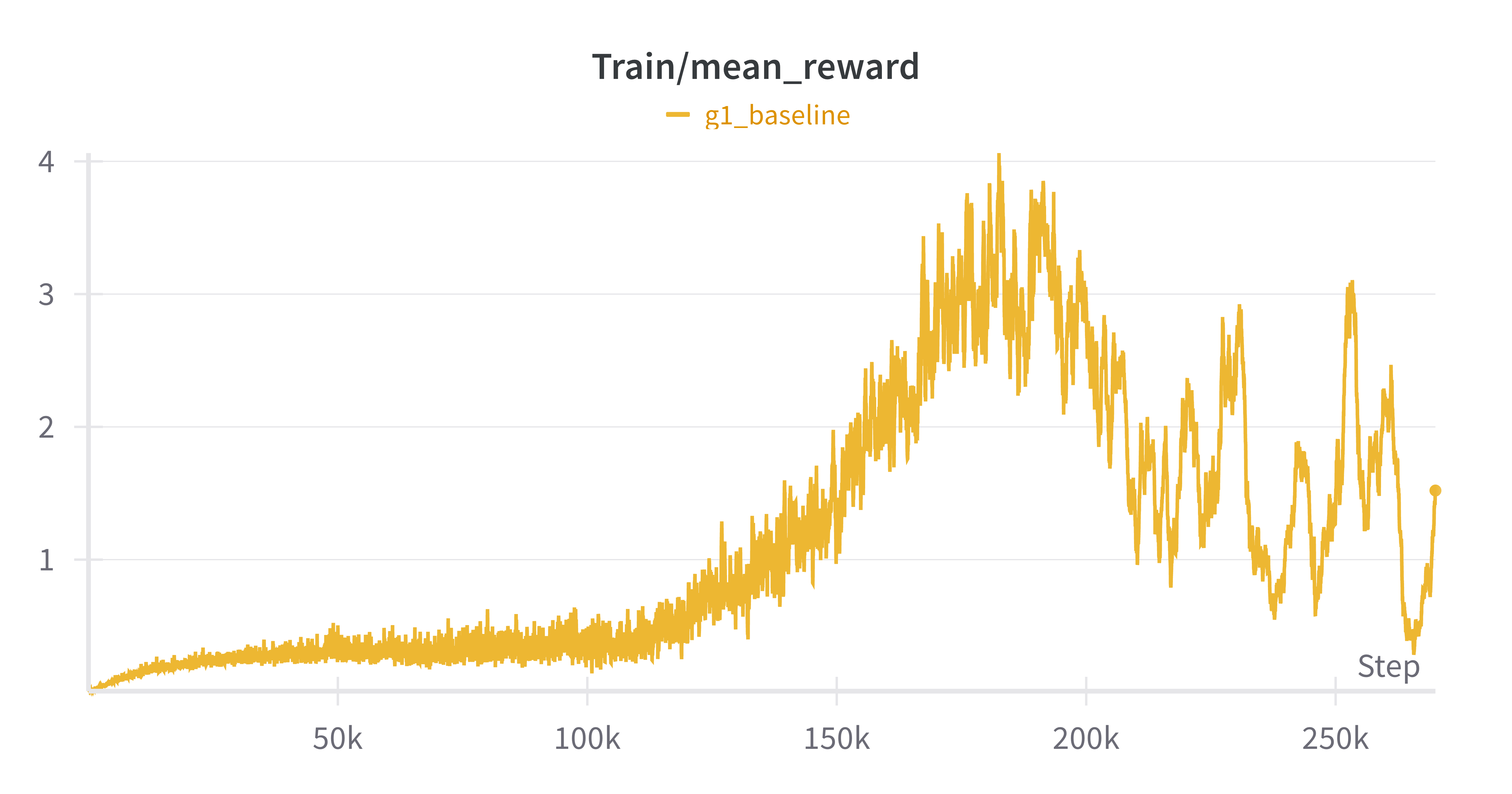
2) Extended Training Run
python legged_gym/scripts/train.py --task=g1 --experiment_name=g1_overnight_full --headless --num_envs=128 --max_iterations=10000 --seed=42
- Parameters: 128 parallel environments, 10,000 iterations, headless mode
- Results:
- mean reward: 1.52 (76x improvement over initial run)
- mean episode length: 579.58 steps (18x improvement)
- training time: ~2 hours (significantly faster than expected)
- key reward components:
- tracking linear velocity: 0.2404 (positive)
- tracking angular velocity: 0.0632 (positive)
- contact: 0.0955 (positive foot contact patterns)
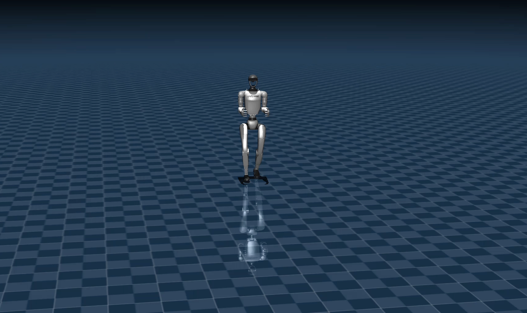
- robot behaviour: stable walking with good balance and response to velocity commands
3) Final Training Run
python legged_gym/scripts/train.py --task=g1 --experiment_name=g1_curiculum --headless --num_envs=96 --max_iterations=15000 --seed=42 --curriculum --domain_rand
- Domain Randomization Improvements
- wider friction range (0.2-1.5) for better terrain adaptation
- added gravity randomization (-1.0 to 1.0) for better balance
- added motor strength randomization (0.8-1.2) for robustness
- more frequent and stronger pushes (every 4s, up to 2.0 m/s)
- Network Architecture
- deeper actor/critic networks [64, 32] instead of single layer
- larger RNN (128 units, 2 layers) for better temporal modelling
- increased initial noise (1.0) for better exploration
- Training Parameters
- reduced environments to 96 (from 128) to allow for larger networks
- increased iterations to 15000 for better convergence
- added gradient clipping and KL divergence control
- more frequent checkpointing (every 100 iterations)
- Reward Structure
- increased tracking rewards (1.2x linear, 1.2x angular)
- stronger penalties for unstable behaviours
- added collision penalty
- increased contact reward (0.25)
- Control Parameters
- increased stiffness and damping for better stability
- higher action scale (0.3) for more dynamic movements
- shorter episodes (20s) for faster learning
Results:
- better generalization through domain randomization
- more stable walking through improved control parameters
- faster learning through optimized reward structure
- better exploration through network architecture changes
Some practical tips/experiments thoughts log
The following are some thoughts I wrote down as a log while writing code to squeeze out performance:
- follow along other world-class projects that have very complex rewards to take inspiration on how to construct the problem
- the best way I found so far to think about RL is generating the data that we’re training on!
- getting codebase to work properly at the beginning is essential, do not skip this step! this includes making sure observation/action numbers are accurate
- metrics to focus on during training: reward per episode, reward length, w&b plots
- train in Isaac lab, validate inside Mujoco for physics, try to apply perturbations or changes
- find the balance between exploration and exploitation: increasing the number of environments increases the policy exploration, and increasing the number of iterations helps with exploitation i.e. refinement of the policy!
- one tip that would be nice with agents: spin up different agents working on different hyper-params tuning to scale experimentation!
- try to interpret the performance of the walking robot in the lens of the reward functions you have, so that you can change your reward function or experiments with a strong intuition vs. adding more exploration/exploitation
- run in headless mode after you’re confident about the training for longer runs to maximize GPU compute and scale your training!
- there’s something about the neural networks size to be extremely small when trained with RL policy, such that it just doesn’t make sense how we’re supposed to fit priors into it. On the good side, this is very effective to run inference. but on the other hand, it looks like we haven’t found a way yet to build intuitions or things like vision policies to train a robot to walk.
- spikes occur and are normal during RL training, the policy is constantly trying new things to find better solutions, which can temporarily decrease performance. also, when curriculum learning is implemented properly things get more challenging as the episode stays for longer or reaches new milestones.
- focus on strong upward trend, values reached in reward/episode length, stability near the end of training i.e. convergence
- observation normalization
- overfit then regularize
Moving Forward
While in this blog we’ve covered the basics of how to train a legged robot to walk and have successfully demonstrated it with code, there are still many open problems and ways in which we can make the policy better in order to learn how to build a production level bipedal controller.
Can you beat the baseline performance? I included sample weights in the log directory.
Methods to Improve Project
The following is a list of ideas to try on to take the existing training code forward:
- Domain Randomization
- terrain (slopes, steps, friction coefficients)
- dynamic parameters (mass, intertia, motor strength, damping properties)
- sensor noise simulation (noise to observations)
- actuator delays (simulate communication/action delays that happen irl)
- Advanced Reward Engineering
- energy efficiency (minimize energy consumption, natural gaits)
- foot clearance (foot clearance during swing phases)
- smoothness (rate of change of acceleration)
- style-based (reference motions from real animals or robots, rewards for matching gaits)
- llm-based rewards: similar to the eureka project, although be careful about what it omits
- Curriculum Learning
- start with simple tasks: standing, then walking on flat terrain
- gradually increase difficulty
- velocity-based curriculum: start with slow movements and then gradually increase target velocities
- robustness training: introduce external pushes of increasing magnitude as training progresses
- Multi-task Learning
- different movement modes: train for walking, trotting, galloping, and recovering from falls
- agility tasks: add jumping, turning in place, or navigating obstacles as additional tasks
- recovery behaviours: specifically train for recovering from unstable states
- Advanced RL Techniques
- hierarchical RL: implement high-level and low-level controllers for better motion-planning
- model-based components: add a dynamics model to improve sample efficiency
- experience replay prioritization: prioritize rare or difficult scenarios during training
- priors: can we leverage priors knowledge before training a controller? i.e. VLAs for manipulation is very popular, can we do the same for bipedal walking?
- Mixture of Experts: to choose between different modes
- Hybrid Controllers: i.e. when can we use MPC when we have models that we think can work well, and when can we use RL when the models might be too hard to run 100 times per second. Then train a model that selects the best action based on what it has currently at hand
- Sim2Real
- deploy in real world, assess performance
- collect failure cases, zoom in the dynamics (i’ve done this with mobile robots)
- online fine-tuning (same exploration methods to fine-tune on real robot)
- real-world RL (reward model like Dyna, learn from failures)
Beyond just improving the learned control policy in this project, there are still many challenging open problems to solve in locomotion in order to build human level controllers.
Open Problems
While building RL controllers to walk is a relatively solved problems, here is a list of some of the most critical problems that can benefit from new approaches to solve:
- terrain-blind generalist gait: one policy that marches from floor to mud to foam to ice
- unified controller that does both planning + control
- seamless gait-switch for all walking scenarios (walking, running, ice, stop)
- vision-conditioned foot placement and walking
- whole body loco-manipulation (walk while holding 10kg, door open, skating that tucks hands)
- reward-engineering: describing things like walk quietly
- language conditioned tasks
- benchmarks for walking performance
- robustness to perturbations and fast resets
- encoding human preferences into walking like arms swinging
- push recovery ≥ 200N in any direction and robot stays up
- zero-shot stair & ladder ascent
- apply behaviour cloning, frame problem as next action prediction with transformers
- using LLMs to write diverse rewards like Eureka
- match human speed ~1.3m/s walk + 3m/s jog
- long path planning like following a map
- energy efficiency CoT (cost of transport) of humans is 0.2, humanoids are at at ~0.4-0.6
- ability to carry different payloads and walk
- use VLA for bipedal walking by learning from human data
- leveraging priors physical knowledge for controllers
Conclusion
In this blog, we covered a deep dive into controlling bipedal humanoids starting from biomechanics to RL, as well as doing an actual experiment training a humanoid Unitree G1 in Isaac Lab and validate in Mujoco.
Hope you learned something new from this blog. If you work on these kinds of problems and have any questions, feel free to reach out!
References
The following are the reference papers and code from the deep dive on bipedal humanoid training and control:
Bipedal
- Berkeley Humanoid: A Research Platform for Learning-Based Control: code uses Isaac Lab, high quality, recent, tested in real world
- Reinforcement Learning for Versatile, Dynamic, and Robust Bipedal Locomotion Control: useful info about the problem of bipedal locomotion and algorithms to solve it
- Real-World Humanoid Locomotion with Reinforcement Learning: from UC Berkeley, quite recent 2024 useful read for practical real world applications
- Humanoid Locomotion as Next Token Prediction, UC Berkeley
- Learning Humanoid Locomotion over Challenging Terrain, UC Berkeley
- The Duke Humanoid: Design and Control For Energy Efficient Bipedal Locomotion Using Passive Dynamics
- Starting on the Right Foot with Reinforcement Learning, Boston Dynamics
- Figure AI RL for Bipedal Locomotion: talks about sim2real, & domain randomization
- How to build Humanoid: Nvidia Isaac Lab: How to Walk: demo of real bipedal bot
- Sim-to-Real Learning of all Common Bipedal Gaits via Periodic Reward Composition: details about crafting reward functions while managing sim2real
- Revisiting Reward Design and Evaluation for Robust Humanoid Standing and Walking: dives a bit deeper into rewards design for robotics
- Reinforcement Learning for Robust Parameterized Locomotion Control of Bipedal Robots: one of the early works by Sergey Levine to teach robots how to walk using RL, plus follow human gaits library
- Learning Locomotion Skills for Cassie: Iterative Design and Sim-to-Real: quite old paper from like 2020, nice read about the general problem of design walking bipedal robots
- Getting SAC to Work on a Massive Parallel Simulator: An RL Journey with Off-Policy Algorithms, Antonin Raffin: tries to use SAC instead of PPO for learning how to walk on quadruped
- FootSteps Planning: Guide with Code
- Deep Reinforcement Learning for Bipedal Locomotion: A Brief Survey: extensive survey about bipedal locomotion
- Feedback Control for Cassie With Deep Reinforcement Learning: talks about learning from human references
- Whole-body Humanoid Robot Locomotion with Human Reference
- Bipedal Walking Papers Collection: recap where research is focused on in recent years
- UC Berkeley Bipedal Publications: some high quality list of publications
- Whole-body Humanoid Robot Locomotion with Human Reference
- Training a humanoid robot for locomotion using Reinforcement Learning (papers + code)
- MoELoco: Mixture of Experts for Multitask Locomotion
- TDMPBC: Self-Imitative Reinforcement Learning for Humanoid Robot Control
- Humanoid Parkour Learning: can walk, run, up/down
- RL and Sim2Real for Manipulation in Isaac Lab
- High-Performance Reinforcement Learning on Spot: Optimizing Simulation Parameters with Distributional Measures: spot RL running, some must-knows for agile control sim2real
- AMO: Adaptive Motion Optimization for Hyper-Dexterous Humanoid Whole-Body Control + code
- CS 294-277: Robots that Learn, UC Berkeley
UniTree
- Unitree RL Gym: RL implementations for UniTree robots in Isaac Gym + Sim2Sim eval Mujoco
- UniTree Mujoco: mainly defines the simulator config stuff
- Isaac Lab: ready H1 training code and environments
- Legged Gym
- Unitree LeRobot
Humanoids Environments
- Mujoco Playground: existing implementations for target robots + GPU parallelization
- HumanoidBench: humanoid benchmark for 15 whole-body manipulation and 12 locomotion tasks in mujoco
- LearningHumanoidWalking: ascending/descending stairs, walking on curves in Mujoco
- Berkely Humanoid: isaac lab code to train bipedal lower body robot
- Humanoid Gym: isaac gym for training + mujoco for sim2sim eval
- learn2walk: sample efficiency of RL algos in mujoco
- DukeHumanoidv1: isaac gym for walking
- HOVER: whole-body controller in teacher-student style. training in isaac lab, and sim2sim eval in Mujoco all on H1-unitree robot
- Human2Humanoid: training in Isaac Gym
- Implementation of Walking robot using Genesis and RL
- HumanoidGym
- LocoMujoco
- AMO: mujoco whole-body control
Cassie Environments
- Cassie RL Walking: trains versatile walking policy for tracking velocity, height, and turning commands, code for berkeley paper
- Gym Cassie: trains Cassie to walk/run forward in MuJoCo, reward for forward motion/penalty jumping
- Gym Cassie Run: rewarded for walking/running forward as fast as possible
- Walking Cassie: after 150 million time-steps, slow/quick forward gaits, lateral and multi-velocity movement
- Gym Cassie: legacy code for OpenAI Gym implementation
- bipedal_walker_terrain: teacher-student model for Cassie in Mujoco
Quadruped Environments
- Learning to Walk using Massively Parallel DeepRL, ETH: takes the idea of extreme parallelism to train in minutes, ramp up terrain difficulty gradually like games, an uneven terrain takes about 20mins to finish training, can use code for inspiration done inside legged_gym, useful since high quality paper and group of people to learn their techniques and work they have done esp. around the Isaac gym for parallelization and domain randomization
- Spot from Boston Dynamics in Isaac Lab + code
- Learning agile and dynamic motor skills for legged robots: AnyMAL from ETH, pioneered RL and sim2real for quadruped robots
- Making Quadrupeds Learning to Walk: From Zero to Hero (code): good for general ideas about what the rewards are, action space, and so on
- Learning Quadrupedal Locomotion over Challenging Terrain, ETH
- Isaac Sim SpeedUp Cheatsheet
RL Libraries
- RSL_RL: code for both Isaac Lab and Legged Gym
- Stable-Baselines3
- Spinning Up RL
- Reinforcement Learning Tips and Tricks: Stable-Baselines3
Books
- Legged Robots that Balance by Marc Raibert: old book from 1980s
- Biomechanics of Movement, Uchida and Delp: strong study of biomechanics
Real World Examples
- Starting on the Right Foot with Reinforcement Learning, Boston Dynamics
- Picking Up Momentum, Boston Dynamics
- Tesla Optimus: natural gait, walking up hills, early demos
- Natural Humanoid Walking using Reinforcement Learning, Figure AI
- Recovery Controller for Booster T1, Kevin Zakka
- 1X World Model Challenge
Misc
- Training AI to play Super Smash Bros
- Eureka: Human-Level Reward Design via Coding Large Language Models
- Voyager: AI agent that plays Minecraft
- MineDojo: open-ended agent learning by watching 100,000s of Minecraft YouTube videos
Notes
-
although in reality, human leg really has around 7-8 DoF not counting toes ↩
-
feel free to try this out in MATLAB ↩
-
Understanding this principle early on, and designing our simulations with maximum domain randomization to capitalize on this observation will be very important as we will later demonstrate ↩
-
checkout my experiments thoughts log ↩